A pod hit the queue. Kubernetes found three candidate nodes. Then, before making a final decision, it did something most engineers don’t realise it can do: it called out to an external HTTP service, asked “which of these would you actually pick?”, and waited for a score.
That HTTP service was the ACO scheduler extender — a FastAPI process running pheromone-weighted placement decisions trained on the Alibaba GPU trace. Kubernetes accepted the score and placed the pod on the node the colony preferred.
No custom scheduler. No cluster-level fork. Just a sidecar and a protocol most people have never needed.
But before the sidecar, there was a paper.
The Research This Builds On
ACO-Adaptive is a cluster scheduler that combines Ant Colony Optimisation with a per-node predictor module for cost-aware, QoS-preserving job placement. The core idea: the colony accumulates pheromone trails across scheduling calls, and a predictor feeds a CostEngine heuristic that penalises nodes forecast to spike before the job lands.
To figure out which predictor to use, the paper ran a 14-way ablation — 10 seeds × 200 latency-critical jobs across a 32-node cluster — comparing deep learning models (LSTM, GRU, TCN, Transformer, MLP), classical time-series methods (ARIMA, linear regression), and signal compression predictors (EMA, moving averages, persistence). The results were submitted to a peer-reviewed systems conference (under review).
The finding that shaped everything after it: EMA with α=0.5 achieved 89.2% safe-node routing versus LSTM’s 75.4% — a 13.8 percentage point gap — with no training cost, no cold-start period, and one line of arithmetic. The simplest predictor in the ablation beat the most complex one. On cluster-level metrics: 28.6% cost reduction over First-Fit on CPU workloads, 97.4% QoS compliance on GPU workloads, P99 scheduling latency below 0.75ms across burst sizes from 1 to 200 concurrent jobs.
A 1-line formula outperformed a trained LSTM by 13.8 percentage points. That result was worth deploying.
The Substack series (Part 1 here) covers the algorithm story — why first-fit scheduling is broken, how the ant colony works, what the 7-benchmark honest scorecard looked like. Everything there ran in Python dicts against the Alibaba 2018 trace.
This post is about what happened when we tried to make it run on a real Kubernetes cluster.
The Protocol Nobody Talks About
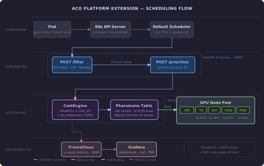
Kubernetes ships with an extension mechanism called the scheduler extender. The idea is simple: after the default scheduler runs its own filtering and scoring passes, it forwards the surviving candidate list to an external HTTP endpoint. Your service scores them and returns a ranked list. Kubernetes picks the winner.
Two endpoints. Two jobs.
POST /filter — receives the full candidate node list and returns a subset. Nodes you reject here never reach scoring. Use it for hard constraints: GPU label present, enough allocatable CPU and memory for the pod’s requests.
POST /prioritize — receives the filtered list and returns a score between 0–10 for each node. Higher scores win. This is where the ACO colony runs.
K8s doesn’t require you to write a new scheduler. It lets you extend the one it already has.
The extender is registered in a KubeSchedulerConfiguration YAML. One stanza, one URL, one flag to mark it as ignorable if the service is down. That’s the entire integration surface.
Filter: Drawing the Hard Lines
The filter endpoint does three checks:
GPU label. If the pod requests a GPU (via nvidia.com/gpu resource), the node must carry an aco/gpu-type label. Nodes without it are rejected immediately and logged to aco_nodes_filtered_total.
CPU headroom. Parse the node’s allocatable CPU (millicores) and the pod’s CPU request. Reject if the node can’t satisfy the request. The parsing handles both "500m" and "2" formats — Kubernetes uses both without warning.
Memory headroom. Same logic, handling Mi, Gi, and bare byte strings.
Nodes that pass all three land in ExtenderFilterResult.Nodes. Nodes that fail go into FailedNodes with a human-readable reason. The Prometheus counter aco_nodes_passed_filter_total tracks the pass rate per node across the session — if a node starts getting consistently filtered, that shows up in Grafana before any SRE notices it in logs.
Prioritize: Where the Colony Runs
Every pod that reaches /prioritize carries a tenant label (scheduling.aco/tenant-id). That label keys into a per-tenant pheromone table — a nested dict, not a global one. Tenant research and tenant prod don’t share memory. Their pheromone trails reflect their own workload histories.
The pheromone table is the colony’s memory. Without per-tenant isolation, a prod burst contaminates the research colony’s priors and vice versa.
For each candidate node, the extender computes a score in two steps.
First, CostEngine.score_node() returns a composite score:
reliability × cost_efficiency × sla_headroom × spike_prediction
reliability comes from the node’s historical selection record. cost_efficiency is derived from the aco/cost-per-hour label — the fleet spans $0.45/hr (T4) to $3.20/hr (V100). sla_headroom measures distance from the pod’s SLA deadline. spike_prediction penalises nodes forecast to saturate before the job lands — this is where the EMA predictor (α=0.5) runs. The ablation found EMA outperformed LSTM by 13.8 percentage points on safe-node routing; accordingly, the extender uses EMA, not a trained model.
Second, that score is multiplied by the current pheromone level for this (tenant, node) pair. The result is normalised to 0–10 for Kubernetes.
After placement, pheromone is updated. All nodes evaporate by ρ=0.05 — trails fade if not reinforced. The winning node gets a deposit of Q/score. A strong placement reinforces the trail; a weak placement deposits less. The colony learns to avoid nodes it had to settle for.
The Import Problem That Took Three Hours
The research repo’s __init__.py eagerly imports WorkloadPredictor, which requires PyTorch. PyTorch takes 8 seconds to load and 2GB of memory. In a K8s sidecar that’s supposed to handle scheduling calls in <1ms, that’s a non-starter.
The fix wasn’t to restructure the research repo (you don’t want to couple production infrastructure to your research codebase). The fix was importlib:
import importlib.util

def _load_module(rel_path: str, name: str):
    path = CORE_DIR / rel_path
    spec = importlib.util.spec_from_file_location(name, path)
    mod = importlib.util.module_from_spec(spec)
    spec.loader.exec_module(mod)
    return mod
This loads cost_engine.py, models.py, and job_models.py directly from their file paths, completely bypassing the package __init__.py. PyTorch never loads. Cold start goes from 8 seconds to under 200ms.
The subtlety: if you later import the same package normally anywhere else in the process, you’ll get two separate module objects and type comparison breaks (isinstance fails across the boundary). The fix is to register the loaded module in sys.modules under its expected package path immediately after loading.
What Pydantic v2 Broke
The extender’s response to /prioritize is a list of (node_name, score) pairs. In the original code, this was modelled as:
class HostPriorityList(BaseModel):
    __root__: List[HostPriority]
Pydantic v2 dropped __root__. Passing this to FastAPI raised a TypeError at response serialisation — not at model definition time, which made it easy to miss in testing. The fix:
from pydantic import RootModel

class HostPriorityList(RootModel[List[HostPriority]]):
    def __iter__(self):
        return iter(self.root)
One more: the CostEngine model enforces gpu_count >= 1 as a Pydantic validator. For non-GPU workloads, the original code passed gpu_count=0, which raised a ValidationError on every CPU-only scheduling call. The fix is to always pass gpu_count=1 — the model uses it only for GPU placement decisions, so the value is irrelevant when gpu_required=False.
Neither of these failures shows up until you run the actual scheduling loop. Both are the kind of thing a typed integration test would catch in 30 seconds.
What the Grafana Dashboard Shows
The local demo runs six simulated nodes across two CPU and four GPU tiers, with three tenants (research, prod, dev) submitting nine workload patterns over a trace replay loop.
The pheromone time series is the clearest signal. At session start, all six nodes sit near the TAU_MIN floor. Within 20–30 scheduling calls, the colony has converged: the A10 node dominates (pheromone ~6.8), CPU and T4 settle in the mid-tier (~5), V100 and P100 sit near zero. The hierarchy is learned from placement outcomes — not configured.
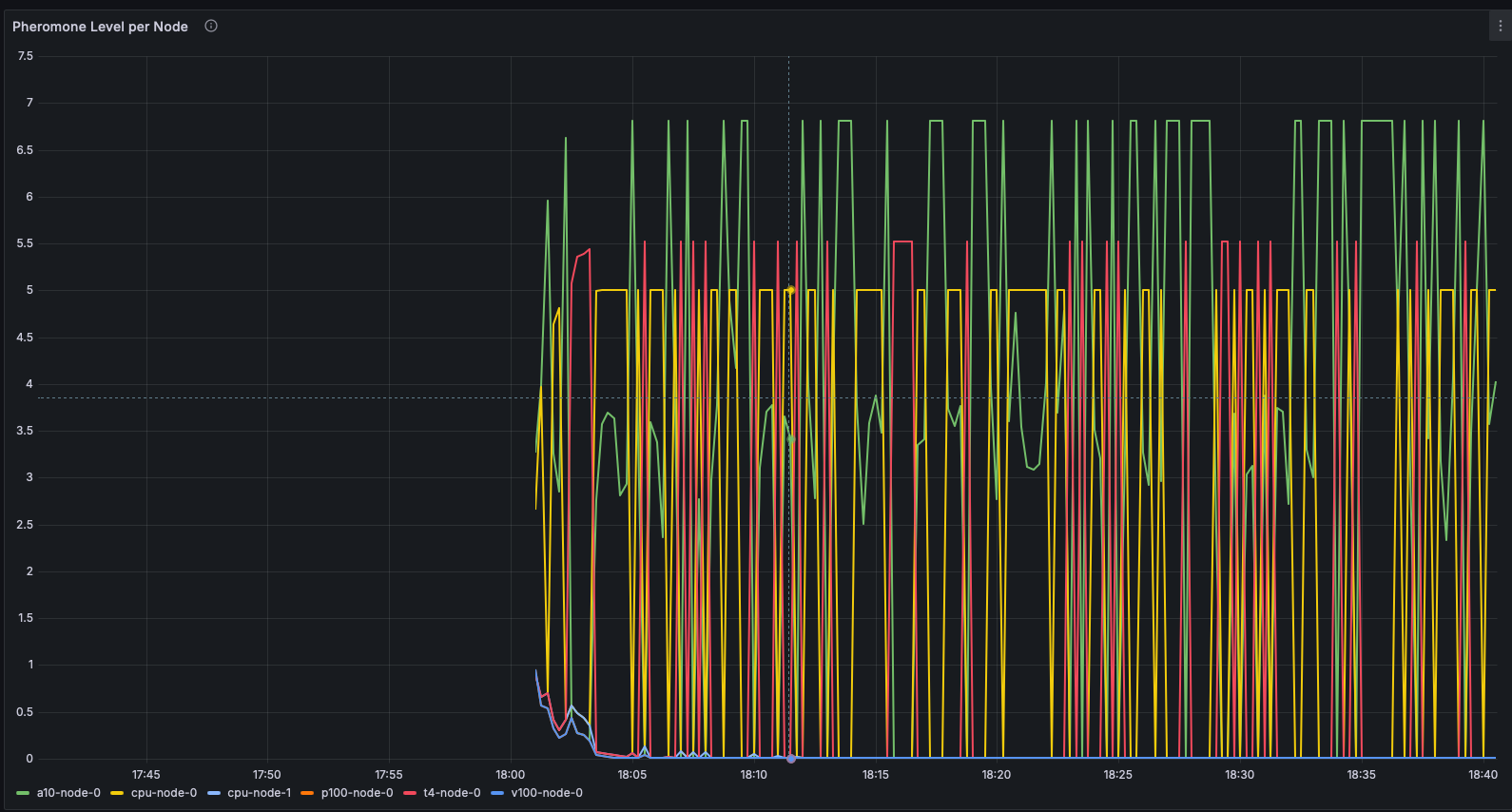
The left half (blank) is before trace replay starts. The lines appear at the reset boundary, then diverge sharply. Colony goes from no information to a stable preference in under 5 minutes.
The cost/job panel tells the same story with dollars. Early in the session, the scheduler occasionally places on the V100 ($3.20/hr) when the A10 ($1.20/hr) would have passed all constraints. After convergence, that doesn’t happen. The colony learnt the cost gradient without any explicit cost rule — it emerged from reinforcement.
The P99 latency panel: flat at sub-millisecond throughout. The ACO scoring loop, pheromone updates, and Prometheus metric writes all complete within the scheduling call window. The extender adds no perceptible latency to pod placement.
The Full Stack
The research paper validated the algorithm on the Alibaba 2018 CPU and GPU traces: EMA α=0.5 at 89.2% safe-node routing, colony P99 below 0.75ms, 28.6% cost reduction. Part 1 of the Substack series told that story in full — the ant colony mechanics, the 14-way ablation, the honest benchmark where spike recall hit 0% because the dataset didn’t have the signal the predictor needed.
What neither the paper nor Part 1 had: a Kubernetes extender, a Prometheus metrics surface, per-tenant pheromone isolation, Terraform-provisioned GPU node pools, or a demo that runs without a GKE cluster. The research established that the algorithm was worth deploying. This is the deployment.
The arc runs: paper (a peer-reviewed systems conference (under review)) → Substack Part 1 (algorithm story) → this repo (K8s infrastructure).
The repo is at github.com/Aravind0403/ACO_Platform_Extension. Local demo runs in three terminals — extender, Prometheus + Grafana, and the trace replay script. No GKE required. The DEMO.md walks through the full session including pheromone reset between runs.
Part 2 of the Substack series covers the build in narrative form — what broke, what the Grafana traces looked like the first time the colony actually converged, and what’s coming next (Redis state store, real K8s pod execution, failure injection). That’s here.
What I want to know: if you’ve built a K8s scheduler extender, where did the protocol actually surprise you? The filter/prioritize split is clean on paper. In practice, the edge cases in GPU label parsing and pheromone initialisation order took longer than the algorithm itself.